Things worth sharing

Do you understand how Apache Iceberg actually works? I have tried to understand it multiple times, but it always felt hard to get into compared to basic Hive tables. When searching for references it often feels more like reading an advertisement with features like: ACID for open file formats, schema evolution and time travel. But even after using Apache Iceberg, I did not grok it before doing practical experiments and sitting down to read the official specification thrice. This post fills the gap of high-level overview and implementation and walks you through the most important features of Apache Iceberg by example, showing you how they work and why they are actually such an huge improvement over Hive tables.

Warning: This post is long and it could take you up to an hour to read it completely.

Apache Iceberg in a nutshell

In its essence Apache Iceberg is a specification of a table format. This means that it specifies how the logical concept of a table, i.e. a 2-dimensional data structure with rows and columns, can be physically stored. This specification contains all necessary information to implement a writer in any programming language that can take columnar data and store it in this table format. But in contrast to encoding data in specific file formats, the output is not just a single file, but multiple hierarchical organized metadata and data files. Complementary, one can implement a reader that understands these files and can read them like a logical table object.

This idea of a table format fits naturally in the process of unbundling database management systems (DBMS), which has been going on for the last ~20 years. In the end a DBMS is just a very complex system, with many interconnected components, that all work together in harmony to allow storing data as tables, that can be manipulated with SQL. In the past components of DBMS have been "cut" from this monolithic system and developed in isolation. Examples of this are query engines like Apache Spark, that combine the query planning and execution part of a DBMS, or open file formats like Apache parquet, that cut off the bottom storage layer, i.e. how data is encoded and compressed.

This process of unbundling components comes with advantages, like freedom from proprietary systems and flexibility of choosing the best compatible systems for the problem at hand. But the obvious disadvantage is, that in this process one has to introduce boundaries between the isolated components. There has been a lot of work to smoothen these boundaries, e.g. via Apache Arrow, but they still make the development of sophisticated features or optimizations that require an overarching view difficult. Two examples for such component spanning features are access methods, i.e. how to most efficiently access the files that are necessary to serve a query, and concurrency control, i.e. how to ensure a consistent view of the data with multiple writers and readers.

Apache Iceberg makes such features possible without the need for a monolithic DBMS structure. It improves on the table abstraction introduced by the data catalog Apache Hive Meta Store (HMS), which boils down to managing table schema, location of data files and partitioning columns. This abstraction was necessary to enable querying data stored in open file formats with SQL, but as we will later see, turned out to be too simple and rigid. Apache Iceberg evolves it by surprisingly reducing the responsibilities of data catalogs. Instead it adds another layer of organization to allow for more sophisticated access of files, consistent concurrent writes and reads and feature like time travel, i.e. reading an older state of a table.

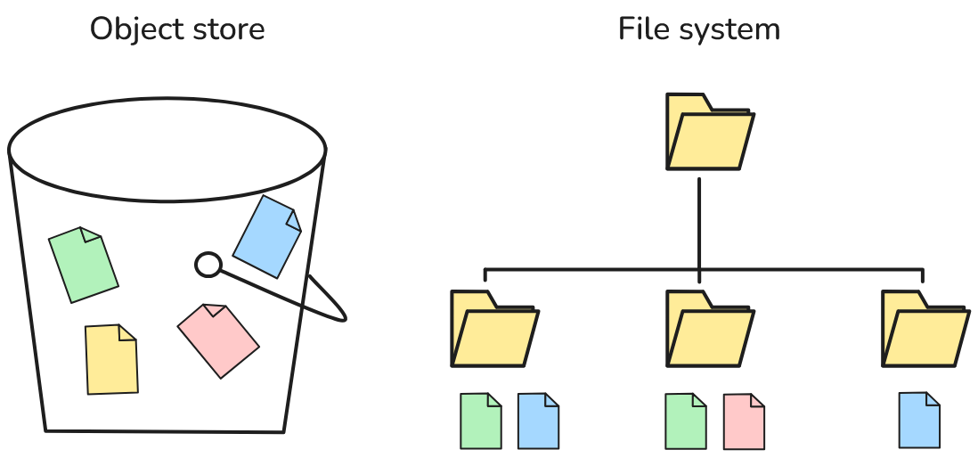
This organization layer is completely file based and only requires in-place writes, seek-able reads and deletes. This way Apache Iceberg can be used on files systems or object-stores, like s3, for easy durability. In spirit of the unbundling, Apache Iceberg does not depend on a single type of open file format to store the actual data, but in theory allows for any format to be used. And finally this organization layer can be used with various data catalogs.

The old Hive way

Before we can appreciate what Apache Iceberg brings to the table (pun!), we must first understand how the table abstraction was initially handled by the HMS.

The HMS is a component of the distributed data warehouse Apache Hive, that enabled SQL queries on top of Apache Hadoop. It is responsible for registering and providing tables by storing metadata about them. This metadata includes (among other things):

Schema: Names and data types of the columns,
Location of the data: In the form of e.g. file paths or URLs. Underlying is a distributed file system or object storage.
Partitions: How the data is split on specific columns without overlaps, e.g. by year.

In short, the HMS is a data catalog and the metadata it stores is necessary for a query engine to understand the underlying data source. When a query engine receives a SQL query, it accesses the HMS to check if the referenced tables even exits, if the selected columns are present, if the expected data types align and if it can use optimizations like partition pruning. Finally the HMS is needed to actually know where the required data of a table can be found by using the stored location metadata.

Hive demonstration

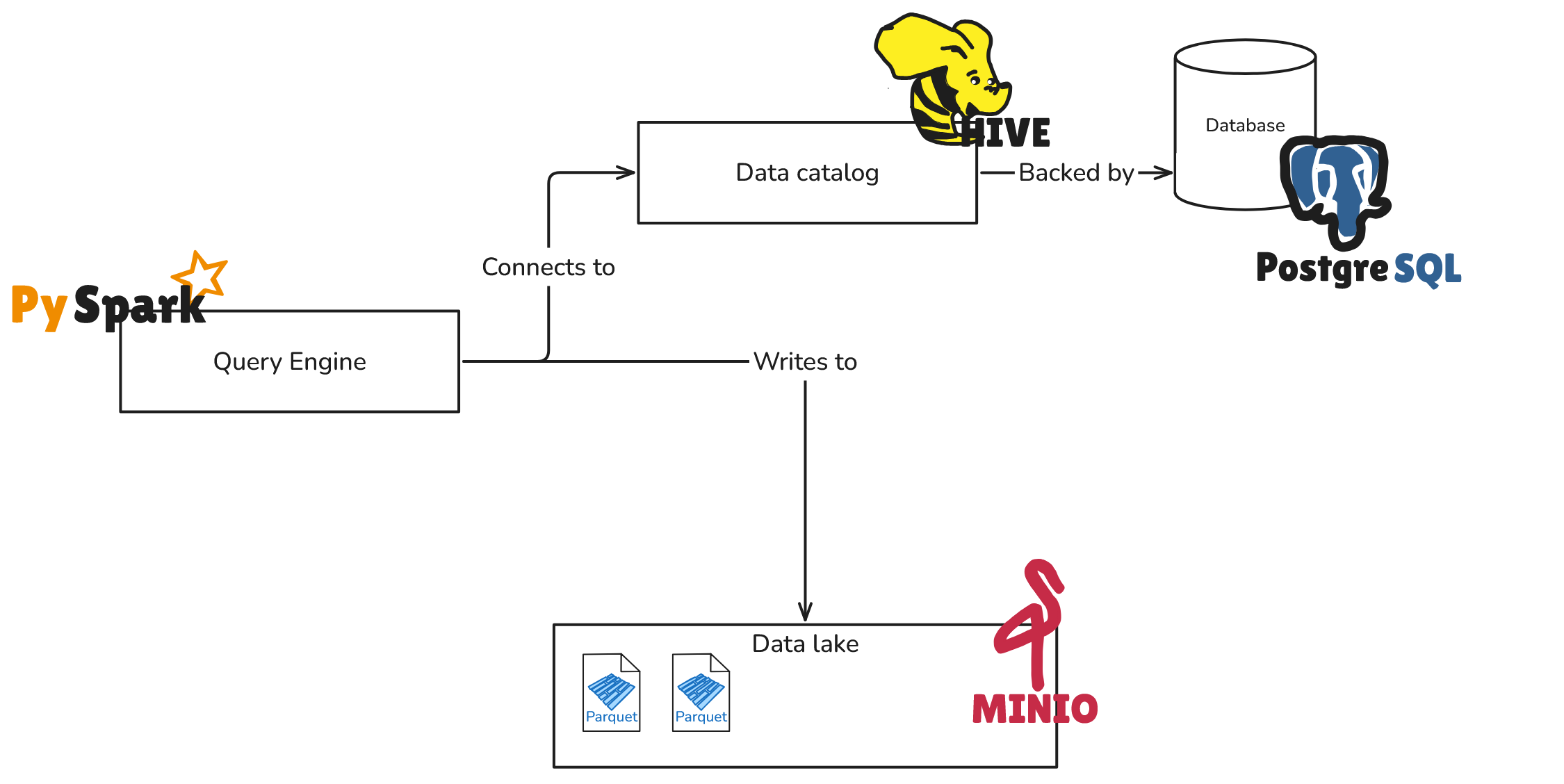
Now for a quick demonstration how this looks in practice. For this we run a HMS instance in a docker container, which under the hood is an Apache Thrift-based server backed by some relational DBMS, in our case a PostgreSQL. To actually interact with the HMS we will be using the query engine PySpark and for storing our data we will use minIO as an object storage, also running in docker. The code to run this yourself can be found here and the setup looks like this:

When all of this is running, we create a table for a small toy dataset of the Marvel X-Men (which we will use throughout the whole blog), using the following schema:

spark.sql("""
CREATE TABLE IF NOT EXISTS xmen (
    id INT,             -- Identifier of the X-Man, e.g. 1
    name STRING,        -- Legal name of the X-Man, e.g. Scott Summers
    alias STRING,       -- The name the X-Man is usally referred to, e.g. Cyclops
    powers STRING,      -- The powers of the X-Man as a comma seperated string, e.g. Optic blasts, team leadership
    birth_year INT      -- The year the X-Man was born, e.g. 1970
)
PARTITIONED BY (active BOOLEAN) -- Is the X-Man still participating in adventures, e.g. true.
STORED AS parquet -- We use parquet as our open file format
LOCATION 's3a://warehouse/xmen' -- Path in our minio object storage
""")

Afterwards we insert some data for active=true X-Men:

spark.sql("""
INSERT INTO xmen PARTITION (active=true) VALUES
    (1, 'Scott Summers', 'Cyclops', 'Optic blasts, team leadership', 1970),
    (2, 'Jean Grey', 'Phoenix', 'Telepathy, telekinesis, Phoenix Force', 1972),
    DISTRIBUTE BY 1  -- Force single file
""""

and then active=false ones:

spark.sql("""
INSERT INTO xmen PARTITION (active=false) VALUES
    (3, 'Hank McCoy', 'Beast', 'Super strength, agility, genius intellect', 1968),
    (4, 'Pietro Maximoff', 'Quicksilver', 'Super speed', 1980),
    DISTRIBUTE BY 1  -- Force single file
""")

From a data lake perspective the result is simple. If we view the minio UI we see two parquet files, nested in the prefix /warehouse/xmen/active=true and /warehouse/xmen/active=false respectively, using the partitioning column active as a hierarchy level.

But what happened in the HMS? To understand this we can access the underlying PostgreSQL, e.g. using DBeaver. Here we are overwhelmed with many tables, you can see a full overview of the HMS database entity relationship diagram here. For a basic understanding the following tables are most important (note that I omit a lot of columns for readability):

TBLS: This holds all the tables that have been registered with the HMS. In our case as we just created a single table it holds the single record:

TBL_ID	SD_ID	TBL_NAME
1	1	xmen

COLUMNS_V2: This table holds all columns that are registered in the HMS, giving their name and data type. We only see the columns for our single table, while the partitioned column active is even missing.

CD_ID	COLUMN_NAME	TYPE_NAME	INTEGER_IDX
1	id	int	0
1	name	string	1
1	alias	string	2
1	powers	string	3
1	birth_year	int	4

PARTITION_KEYS: This holds the partition column, which was missing from the COLUMNS_V2 table:

TBL_ID	PKEY_NAME	PKEY_TYPE	INTEGER_IDX
1	active	boolean	0

PARTITIONS: This holds all partitions that have been created. In our case we have a single boolean partition column, hence two records are present that are linked to our table via TBL_ID:

PART_ID	PART_NAME	SD_ID	TBL_ID
1	active=true	2	1
2	active=false	3	1

SDS: Standing for "storage descriptors" this table holds the locations in the data lake where the associated data for our table lives. We have three records, the first being the highest hierarchy level giving the path prefix to all data files of the table, and two records for each partition one.

SD_ID	LOCATION	CD_ID
1	s3a://warehouse/xmen	1
2	s3a://warehouse/xmen/active=true	1
3	s3a://warehouse/xmen/active=false	1

Represented as a very simplified entity relationship diagram, this looks like this:

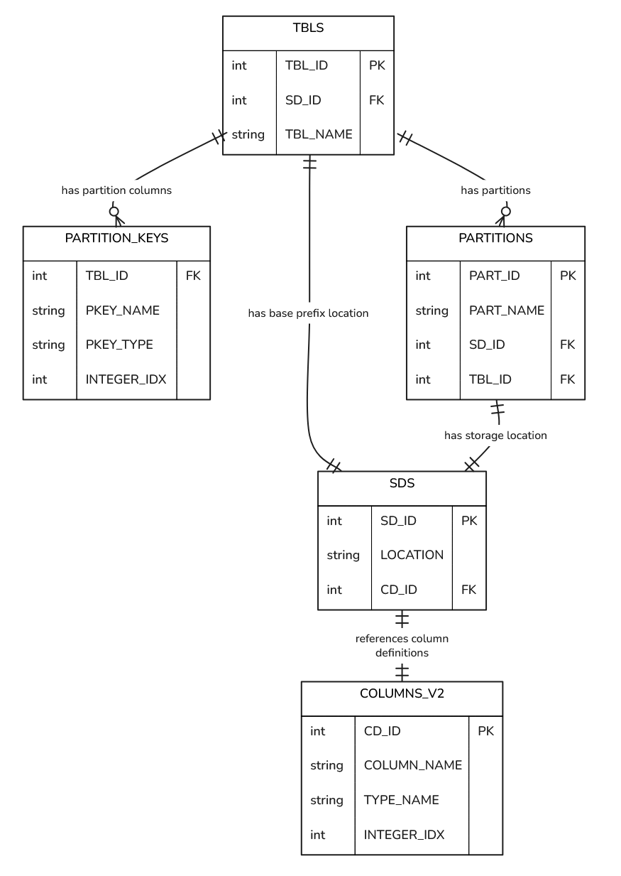
With this in mind we can formulate the HMS table abstraction as: A table is an entity that has an associated base prefix location under which all of its data is stored. Additionally it can have partitions, each with an associated prefix location lower in the hierarchy than the base prefix location. Finally, the schema of a table is connected to its storage locations and not directly to the table.

Let's see what this table abstraction has for implications in practice. Imagine we run the following query

select name, powers
from xmen
where active = false

with our query engine. The query engine would then need to get information from the HMS on how to actually execute this query, i.e. create a query plan. This process could look something like this, first TBLS must be checked if the table xmen does even exists. Then PARTITION_KEYS is used to check if the column active used in the predicate filter (where clause) is a partitioning column. In our case it is, which allows the query engine to get only the prefix location for the requested partition value from the table SDS via the PARTITIONS table. Finally it can validate if all the columns requested in the projection, i.e. name and powers, are present by querying COLUMNS_V2.

After this is done the query engine knows if the query can be answered and if so, where the data resides that it must scan. But here lies a fundamental shortcoming of the HMS approach, because to actually plan the tasks that need to be executed the query engine must know exactly what files need to be scanned. This means that for every data location, it must list all files that sit behind it, e.g. for s3 using the API call ListObjectsV2. Hence, the time it takes to find all files scales with the number of locations to scan and files behind each one, as not all files can be listed in a single API call. With a latency around 200 ms per API call for cloud storage, this means that depending on the size of a table, how many partitions it has and how its files are compacted, a query engine could spend multiple minutes just listing files to plan how to execute a query, without actually touching the data once. This shortcoming was the main reason why Netflix even invented Apache Iceberg back in 2017, and soon we will see how they solved it.

Other shortcomings

Besides the listing of files problem there are many other things that one may want to do with a table abstraction that are either cumbersome or not possible with the Hive style. For example:

How could we delete or update a single row in a table? In the Hive style the only way is to overwrite either a single partition, where the row is located, or the whole table. For big tables this can be a huge operation for a tiny change.
What happens when a reader scans a table, while a parallel write adds files? Per default this could result in the reader seeing data that was written after they started their query (dirty read) or even an inconsistent state. (Note, that this issue was later addressed by introducing Hive transactions.)
What happens if we want to evolve the schema? For adding new columns old data will just produce nulls. But for more complex schema changes like removing, renaming or reordering columns issues arise.
What happens if we want to use spaces in the partitioning values? As the partitions are integrated in the file path or URL, issues can arise with spaces, slashes or other special characters.
What happens if we want to change the way the data is partitioned? In the Hive style we would need to rewrite all the data of a table.
What could we do to look at an older state of the data? In the Hive style there exists only one version of the table, the current one. If we want to have a history, we would need to either add this in the data model, e.g. by using slowly changing dimensions, or store a copy of the full table for a point in time of the granularity we want, e.g. partitioning by year, month and day. This either introduces a lot of complexity or wastes storage.

All the above shortcomings can be traced back to the simple design of the HMS table abstraction. While the approach of a table being a pointer to a directory or prefix and modeling partitions directly in the path hierarchy is intuitive and easy to reason about, it reduces flexibility and makes some operations expensive. With this tradeoff established let's deep dive in to the design of Apache Iceberg to understand how it introduced a complex organization layer to overcome these shortcomings.

Core ideas

Apache Iceberg used the following two core ideas for its table abstraction:

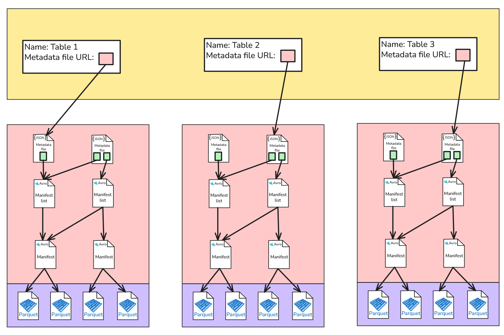
Pull most of the metadata responsibility out of the data catalog. For Apache Iceberg tables the data catalog only stores the table name and a file path/URL to a file that holds the actual metadata, which can be atomically switched the table has changed. This drastically reduces the load on the data catalog and allows for easy compatibility with various catalogs.
Introduce a new metadata layer that is entirely based on immutable files, which sits on top of the files that actually store the data, i.e. data files. Here hierarchical ordered files define the table and state how the data files should be interpreted. This decouples the physical storage of data from its logical interpretation, which yields a lot of flexibility.

With this change the logical representation of a table is spread across three layers:

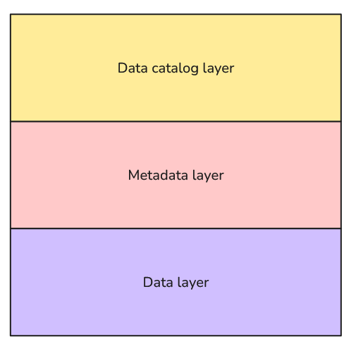
Let's look at the responsibilities and components of these layers from the bottom up. But note, that this will be a simplified view and details will be covered afterwards with examples.

The data layer

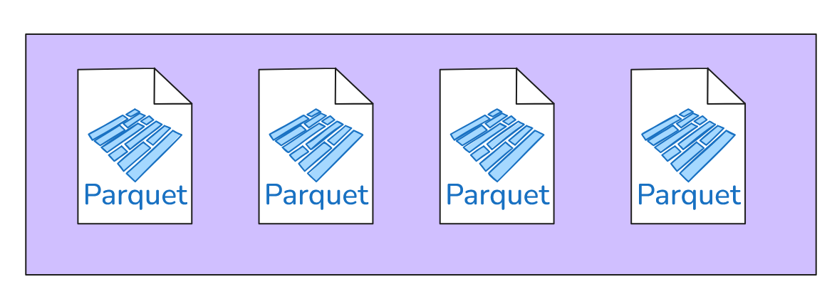
In this layer the actual data that make up a table is stored in separate files. Here no restriction on the actual format of these data files is given by Apache Iceberg and in theory any format could be used or even various once used for a single table. But in practice the common implementations support Apache parquet, Apache ORC, Apache Avro or the Puffin file format.

It is important to note here, that a table is not given by simply combining all data files at this layer. They simply serve as building blocks, where the metadata layer is the manual that shows how to combine them. This means that deprecated files that are no longer part of a table can still be present here, but will simply be ignored on a read. Later we will see that data files can in fact represent rows that were deleted from a table and then be used to remove rows from other data files on a read.

When a writer modifies an Apache Iceberg table, e.g. by appending rows to it, it first writes the data files. Afterwards it moves up to the metadata layer to write metadata files to give the data files meaning. If something goes wrong while the metadata is written, e.g. a concurrency conflict with another writer, the data files do not need to be rewritten and the process can just be restarted. This is great, because writing data files should take up the majority of time and would be wasteful to repeat.

The metadata layer

The metadata layer is the core of Apache Iceberg and fully described in the specification. It consists of the following components:

Metadata files
Snapshots
Manifest lists
Manifest files

which are hierarchically ordered, with the final goal to map many data files to a single logical table abstraction.

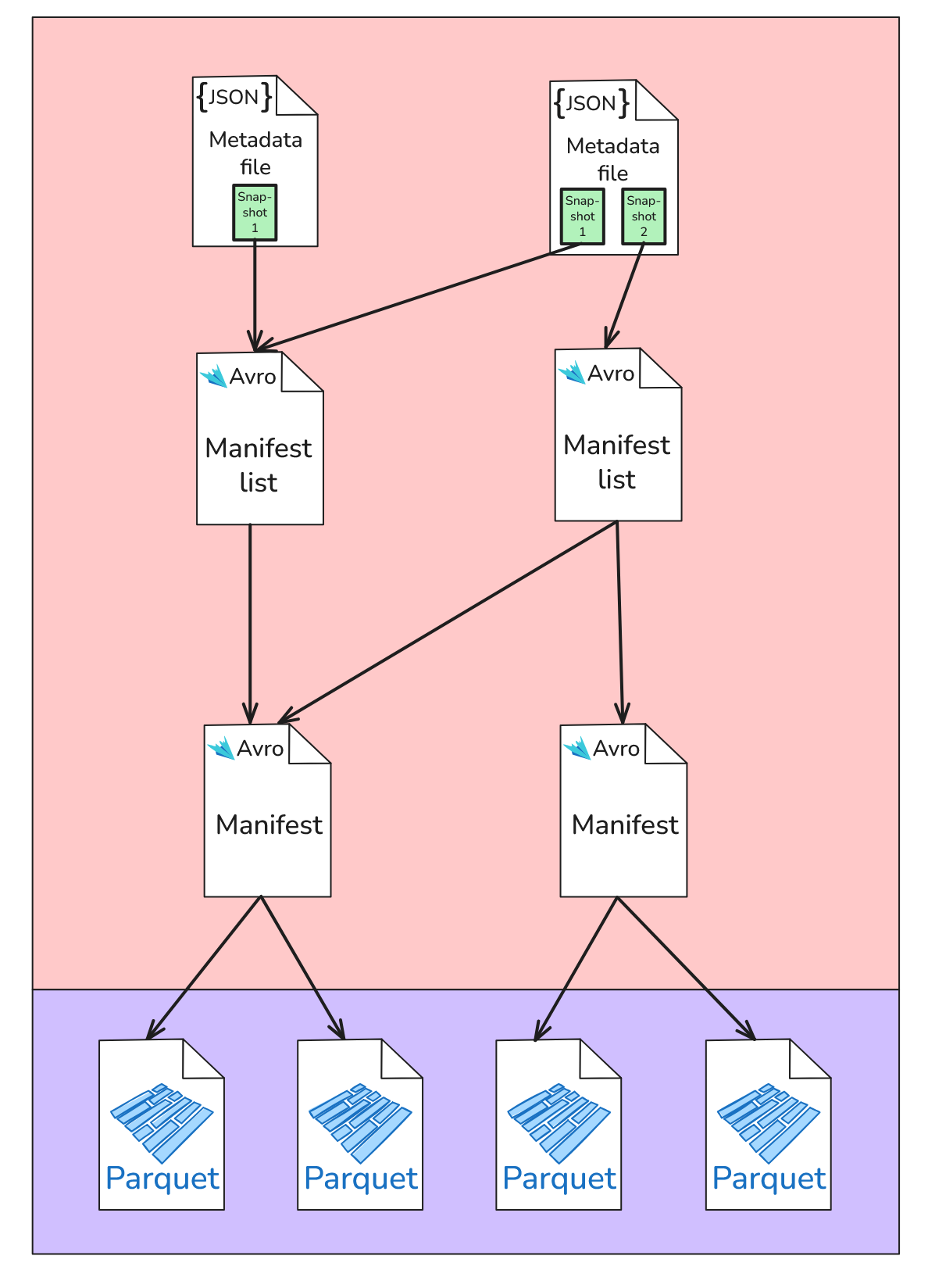
A metadata file is a JSON file that represents a version of a table. It holds all snapshots that are valid for a table version.

A snapshot is a representation of a table at a point in time and points to a manifest list. It is stored in a metadata file.

A manifest list is an Avro file that groups manifest files.

A manifest file is an Avro file that simply groups and describes data files. It therefore acts as the connection of the metadata layer with the data layer.

At this point it becomes clear where the name Iceberg stems from. Like an iceberg where 90% of its volume is hidden below the surface, an Iceberg table has all of these files hidden below it.

To circle back to the appending rows example, after a writer has written data files to modify a table it must then write one or more manifest files that group and reference them. Then it must create a new manifest list that contains the new manifest files. Finally it must create a new metadata file based on the previous one that contains a new snapshot that points to the new manifest list file.

Complementarily, a reader must be able to obtain a list of all data files that make up a table by first reading the metadata file and selecting a snapshot of choice. Then reading the corresponding manifest list file and all the manifest files that are grouped in it, to then finally extract all data files locations from it.

At this point we can already see one of the Hive style shortcomings eliminated: The listing of data files problem. Instead of running multiple ListObjectsV2 API calls to obtain thousands of data file locations, now they can just be extracted from a few manifest files. This of course assumes that every manifest file lists many data files and we do not end up with a 1:1 mapping, an issue that we will discuss later. With this it also becomes clear why the row-by-row based file format Avro is used for the manifest files, as the data files metadata is extracted sequentially from them.

The data catalog layer

The data catalog layer has two simple responsibilities. First it must store a location, e.g. URL, for every table that points to its current metadata file. This location is used by writers or readers as an entry point when writing to or accessing a specific table. Second it must allow to atomically swap this metadata file location with one that points to a new version. This is used by writers when a table is modified.

For the swapping optimistic concurrency control is used to ensure consistency when multi writers modify a table in parallel. This means that conflicts, i.e. writes at the same time, are considered to be rare. Hence a write will just write all data and metadata layer files and only at the final step check, if no other write has updated the metadata file location in the meantime. For this it only swaps the old location with the new one using a compare and swap operation, i.e. if the old location is still what it expects and used to build the new metadata file.

Note here, that the data catalog layer can be implemented by various compatible types, that may be harder or easier to deploy and maintain or come with extra features.

Examples

With this basic mental model on how Apache Iceberg works established, let's look at a few examples showcasing features and explain how the different layers make them work. If you want to follow along you can find the code of the examples here.

Example: Create an Iceberg table and show file structure

The first thing we are going to do is create an Iceberg table and have a deeper look at the metadata layer. For this we will be using PyIceberg and for our data catalog we use an sqlite database for simplicity.

from pyiceberg.catalog import load_catalog

catalog = load_catalog(
    # Name of the catalog. One can store multiple catalogs in the same database.
    "marvel",
    **{
        # We will use the SQLCatalog type.
        "type": "sql",
        # Gives the location of the sqlite database.
        "uri": f"sqlite:////tmp/warehouse/pyiceberg_catalog.db",
        # Gives the path were the metadata and data of the tables will be stored.
        "warehouse": f"file:///tmp/warehouse",
    },
)

This will create the sqlite database pyiceberg_catalog.db in the /tmp/warehouse/ directory. 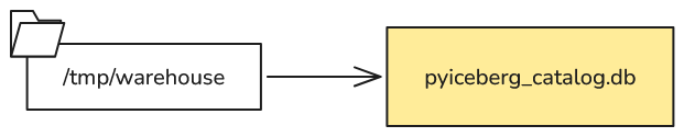Inside this directory we can have a first look at our data catalog using sqlite3 ./pyiceberg_catalog.db and

sqlite> .tables
iceberg_namespace_properties  iceberg_tables

We can now create namespaces in this catalog. Namespace are used to hierarchically group tables and are useful to avoid name conflicts. One can give them properties, which can be useful for giving more information, like description or owner, or to give a specific location where the data of this namespace shall be stored. Let's create one namespace for the X-Men

catalog.create_namespace_if_not_exists(
    "xmen",
    properties={
        "description": "Mutant superheroes with powers",
        "owner": "professor_x",
        "location": f"file:///tmp/warehouse/xmen",
    },
)

We can now see in the data catalog:

sqlite> select * from iceberg_namespace_properties;
catalog_name  namespace  property_key  property_value
------------  ---------  ------------  ------------------------------
marvel        xmen       description   Mutant superheroes with powers
marvel        xmen       owner         professor_x
marvel        xmen       location      file:///tmp/warehouse/xmen

Now let's create our first Iceberg table. For this we first load a csv of X-Men characters as an arrow table,

from pyarrow.csv import read_csv

df = read_csv("./x-men.csv")

which looks like this:

id	name	alias	powers	birth_year	active
1	Scott Summers	Cyclops	Optic blasts, team leadership	1970	TRUE
2	Jean Grey	Phoenix	Telepathy, telekinesis, Phoenix Force	1972	TRUE
3	Logan	Wolverine	Regeneration, adamantium claws	1880	TRUE
...

Then we can create a table using:

table = catalog.create_table(
    identifier="xmen.characters",
    schema=df.schema,
)

Afterwards our filesystem structure has changed to: and we have our very first metadata file, 00000-<uuid-a>.metadata.json. Note here that I shortened the filename for readability, and will do so for all other files. For metadata files the filename follows the pattern <version_number>-<UUID>.metadta.json, where version_number is 5-digit zero padded and increases with every commit, i.e. change of the table.

Meanwhile in our data catalog we now have a row in the iceberg_tables table:

sqlite> select * from iceberg_tables;
catalog_name  table_namespace  table_name  metadata_location           previous_metadata_location
------------  ---------------  ----------  --------------------------- --------------------------
marvel        xmen             characters  file:///tmp/warehouse/xmen/
                                           characters/metadata/
                                           00000-<uuid-a>.metadata.json

If we inspect the JSON file we see (shortened)

{
  "location": "file:///tmp/warehouse/xmen/characters",
  "table-uuid": "037f79f9-1e57-4a8e-bb25-f173924c3e3c",
  "last-updated-ms": 1754402272360,
  "last-column-id": 6,
  "schemas": [
    {
      "type": "struct",
      "fields": [
        {
          "id": 1,
          "name": "id",
          "type": "long",
          "required": false
        },
        {
          "id": 2,
          "name": "name",
          "type": "string",
          "required": false
        },
        [...]
      ],
      "schema-id": 0,
      "identifier-field-ids": []
    }
  ],
  "current-schema-id": 0,
  "partition-specs": [
    {
      "spec-id": 0,
      "fields": []
    }
  ],
  "default-spec-id": 0,
  "last-partition-id": 999,
  "properties": {},
  "snapshots": [],
  "snapshot-log": [],
  "metadata-log": [],
  "sort-orders": [
    {
      "order-id": 0,
      "fields": []
    }
  ],
  "default-sort-order-id": 0,
  "refs": {},
  "statistics": [],
  "format-version": 2,
  "last-sequence-number": 0
}

Don't get lost in the details. Some things immediately catch the eye, e.g. we have a location like in Hive style and a list of schemas, but the amount of metadata is at first overhelming. The important part is that this structure already promises that a lot of metadata will be stored on an Iceberg table, and we will gradually understand some of the fields down the line.

Next, we want to insert data into our table. For this we just append our data frame:

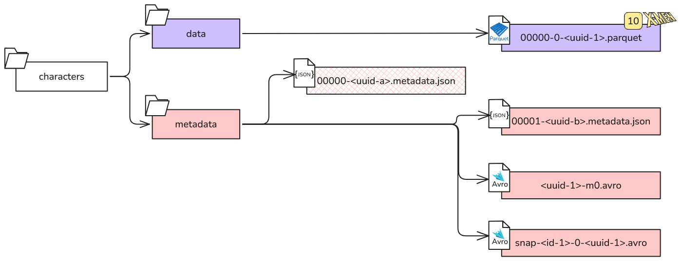
table.append(df)

This results in four new files in our filesystem, three in the metadata layer and one in the data-layer:

And inside our data catalog, we see that the metadata location has changed:

sqlite> select * from iceberg_tables;
catalog_name  table_namespace  table_name  metadata_location            previous_metadata_location
------------  ---------------  ----------  ---------------------------- ----------------------------
marvel        xmen             characters  file:///tmp/warehouse/xmen/  file:///tmp/warehouse/xmen/
                                           characters/metadata/         characters/metadata/
                                           00001-<uuid-b>.metadata.json 00000-<uuid-a>.metadata.json

The current metadata location now points to the new metadata file 00001-<uuid-b>.metadata.json, notice the increment in the version number, while the previous location points to the old one. This shows that in the process of appending data to the table we have not just written new data and metadata files, but done an atomic commit in our data catalog to change this. This atomic commit is responsible for making all newly written data "visible" for the table, because for any reader the table is just what the metadata file states.

Let's inspect this on a deeper level and first look at the most important part that changed when going from version 00000 to 00001. In version 00000 we had an empty list of snapshots:

"snapshots": [],

while in 00001 we now have this:

"snapshots": [
     {
       "snapshot-id": <id-1>,
       "sequence-number": 1,
       "timestamp-ms": 1754402715529,
       "manifest-list": "file:///tmp/warehouse/xmen/characters/metadata/snap-<id-1>-0-<uuid-1>.avro",
       "summary": {
         "operation": "append",
         "added-files-size": "2846",
         "added-data-files": "1",
         "added-records": "10",
         "total-data-files": "1",
         "total-delete-files": "0",
         "total-records": "10",
         "total-files-size": "2846",
         "total-position-deletes": "0",
         "total-equality-deletes": "0"
       },
       "schema-id": 0
     }
   ]
"current-snapshot-id": <id-1>,

Here we observe two things, first we now have a snapshot in our snapshots list, and like previously stated, a snapshot represents a table at a point in time. We can see that a snapshot has a snapshot-id, to uniquely identify it, and that it contains information on the last operation that was used to create it, in our case we did an append for 10 X-Men. But most importantly a snapshot points to a manifest list file, in our case snap-<id-1>-0-<uuid-1>.avro, which we will look into more detail soon.

Second, the metadata file now has a field called current-snapshot-id, which gives the id of the snapshot that is currently "active" for this table. In our case it is simply the most recently created, and only, snapshot. This field is used when a reader loads the metadata JSON to identify what snapshot is active and hence what manifest list file it must load next.

Speaking of the manifest list file, let's examine it next. Regarding its filename it follows the pattern snap-<snapshot_id>-<attempt>-<commit_uuid>.avro, where snapshot_id is the id of the snapshot, attempt starts at 0 and is incremented for every conflict when attempting to change the location in the data catalog, and commit_uuid is the UUID associated with the commit. To inspect it we can use avro-tools and jq,

alias avro-tools='java -jar ~/tools/avro-tools-1.11.3.jar'
avro-tools tojson "snap-<id-1>-0-<uuid-1>.avro" | jq

which gives the following:

{
  "manifest_path": "file:///tmp/warehouse/xmen/characters/metadata/<uuid-1>-m0.avro",
  "manifest_length": 4655,
  "partition_spec_id": 0,
  "content": 0,
  "sequence_number": 1,
  "min_sequence_number": 1,
  "added_snapshot_id": <id-1>,
  "added_files_count": 1,
  "existing_files_count": 0,
  "deleted_files_count": 0,
  "added_rows_count": 10,
  "existing_rows_count": 0,
  "deleted_rows_count": 0,
  "partitions": {
    "array": []
  },
  "key_metadata": null
}

Ignoring the metadata for the moment, the most important part is the field manifest_path pointing to a manifest file. And if we inspect the manifest file using:

avro-tools tojson "<uuid-1>-m0.avro" | jq

we see:

{
  "status": 1,
  "snapshot_id": {
    "long": <id-1>
  },
  "sequence_number": null,
  "file_sequence_number": null,
  "data_file": {
    "content": 0,
    "file_path": "file:///tmp/warehouse/xmen/characters/data/00000-0-<uuid-1>.parquet",
    "file_format": "parquet",
    "partition": {},
    "record_count": 10,
    "file_size_in_bytes": 2846,
    "column_sizes": {
        [...]
    },
    "value_counts": {
        [...]
    },
    "null_value_counts": {
        [...]
    },
    "nan_value_counts": {
      "array": []
    },
    "lower_bounds": {
      "array": [
            [...]
        {
          "key": 3,
          "value": "Beast"
        },
            [...]
      ]
    },
    "upper_bounds": {
      "array": [
            [...]
        {
          "key": 3,
          "value": "Wolverine"
        },
            [...]
      ]
    },
    "key_metadata": null,
    "split_offsets": {
      "array": [
        4
      ]
    },
    "equality_ids": null,
    "sort_order_id": null
  }
}

Here I have omitted many fields for readability, but the key insight is that the manifest file lists data files. In our case it stores just one, 00000-0-<uuid-1>.parquet, which follows the filename pattern 00000-<task_id>-<commit_uuid>.parquet, where task_id is specific to the writer used to create it. Additionally, it stores metadata information on the data inside those data files, e.g. lower_bounds and upper_bounds give the bound values for each column. For example for the name field, which has the id 3, we can see that the data file 00000-0-<uuid-1>.parquet contains on the lower bound the X-Man "Beast" and on the uppper "Wolverine". If we would be looking for the X-Man "Angel", which is not included in this range, we instantly know that we could skip this data file. This technique is called pruning and becomes very efficient in Apache Iceberg, because we can directly prune from the manifest file level, without having to query the individual underlying data files metadata.

To summarize our table is given by the following file hierachy: 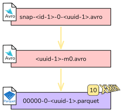which a reader just traverses to collect all data files that make up the current state of a table.

For the following examples, if not stated otherwise, we will use this state as a base to showcase other features.

Example: Append more X-Men

As a simple next example we just add three more X-Men to our table. We can simply do this using:

df = read_csv("./x-men2.csv")
table = catalog.load_table(identifier="xmen.characters")
table.append(df)

Looking at the filesystem structure we see the same result as for the first append: three more metadata files and one data file.

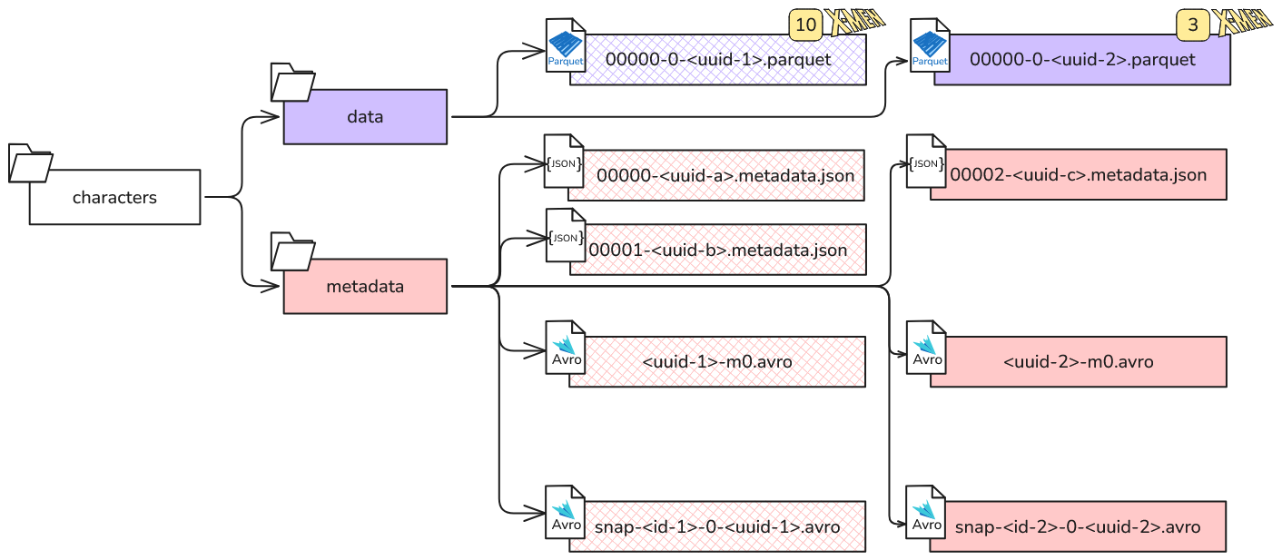
But in contrast, the now active manifest list file does not only point to one manifest file, but two:

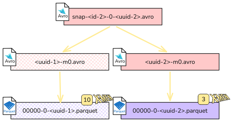
The idea stays the same: A reader loads the manifest file and traverses all child manifest files and associated data files to get the current state of the table. While it may seem wasteful that a simple append produces that many files, this wastefulness is exactly what gives Apache Iceberg its powers. Because now we not only see the current state of the table, but have the information what operations where done in what order to get to this state, see for example what the snapshot list of the metadata file 00002-<uuid-c>.metadata.json looks like:

"snapshots": [
  {
    "snapshot-id": <id-1>,
    "sequence-number": 1,
    "timestamp-ms": 1754402715529,
    "manifest-list": "file:///tmp/warehouse/xmen/characters/metadata/snap-{id-1}-0-<uuid-1>.avro",
    "summary": {
      "operation": "append",
      "added-files-size": "2846",
      "added-data-files": "1",
      "added-records": "10",
        [...]
    },
    "schema-id": 0
  },
  {
    "snapshot-id": <id-2>,
    "parent-snapshot-id": <id-1>,
    "sequence-number": 2,
    "timestamp-ms": 1754405155465,
    "manifest-list": "file:///tmp/warehouse/xmen/characters/metadata/snap-{id-2}-0-<uuid-2>.avro",
    "summary": {
      "operation": "append",
      "added-files-size": "2571",
      "added-data-files": "1",
      "added-records": "3",
        [...]
    },
    "schema-id": 0
  }
],

Example: Delete an X-Man

In this example we want to delete an X-Man from the table, because their existence was eliminated from all timelines. Without Apache Iceberg we would need to do the following:

Find the file were the X-Man is stored.
Load it into memory.
Delete the record of the X-Man we want to delete.
Overwrite the original file, now without the deleted record.

Depending on the table setup this could result in either loading a single file, loading many files that belong to a single partition or loading all files that belong to the table. Hence, for big tables and a number of records to be deleted this can be a wasteful operation. While the way our table is partitioned could limit the overwrite to only a few partitions, the deletion of a single row from a table with several giga byte large partitions still involves large unnecessary data movements.

Apache Iceberg solves this issue by not actually deleting records in the data files, but by adding the concept of a delete file. A delete file shares a lot of similarities with a data file, but instead of describing records that are "added" to a table, it describes records that are "removed". They therefore act like a filter to remove records from previously added data files.

Copy-on-write

Let's look at an example, where we will use PySpark, because PyIceberg does not support writing delete files yet. We first create a SparkSession that is connected to our already existing sqlite data catalog

from pyspark.sql import SparkSession

spark = (
    SparkSession.builder.appName("deleting-x-man")
    # Iceberg packages
    .config(
        "spark.jars.packages",
        "org.apache.iceberg:iceberg-spark-runtime-4.0_2.13:1.10.0,"
        "org.xerial:sqlite-jdbc:3.46.0.0",
    )
    # Configure catalog to use SQLite via JDBC
    .config(
        "spark.sql.extensions",
        "org.apache.iceberg.spark.extensions.IcebergSparkSessionExtensions",
    )
    .config("spark.sql.catalog.marvel", "org.apache.iceberg.spark.SparkCatalog")
    .config("spark.sql.catalog.marvel.type", "jdbc")
    .config(
        "spark.sql.catalog.marvel.uri",
        "jdbc:sqlite:////tmp/warehouse/pyiceberg_catalog.db",
    )
    .config("spark.sql.catalog.marvel.warehouse", "file:///tmp/warehouse")
    .getOrCreate()
)

Then we delete the unlucky Cyclops by id

spark.sql("DELETE FROM marvel.xmen.characters WHERE id = 1")

The filesystem structure now shows the following:

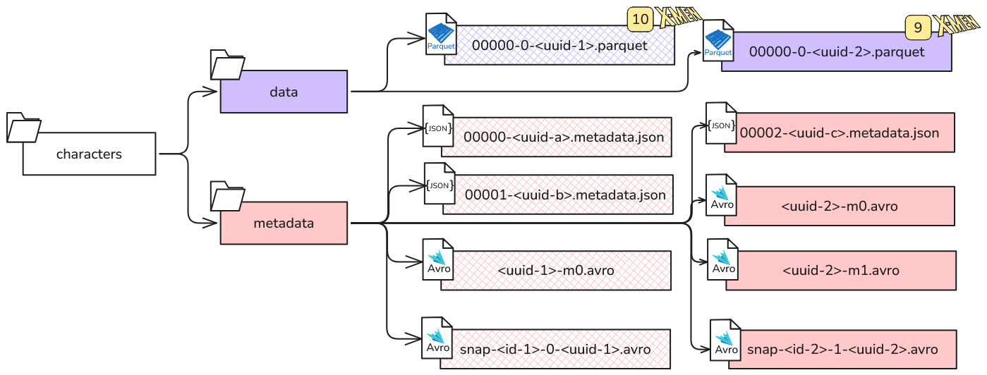
No delete file written! Instead, if we inspect the latest snapshot, we see that it points to the two new manifest files.

{
  "manifest_path": "file:/tmp/warehouse/xmen/characters/metadata/<uuid-2>-m1.avro",
  "manifest_length": 7373,
  "partition_spec_id": 0,
  "content": 0,
  "sequence_number": 2,
  "min_sequence_number": 2,
  "added_snapshot_id": 48153905500596197,
  "added_files_count": 1,
  "existing_files_count": 0,
  "deleted_files_count": 0,
  "added_rows_count": 9,
  "existing_rows_count": 0,
  "deleted_rows_count": 0,
  "partitions": {
    "array": []
  },
  "key_metadata": null
}
{
  "manifest_path": "file:/tmp/warehouse/xmen/characters/metadata/<uuid-2>-m0.avro",
  "manifest_length": 7371,
  "partition_spec_id": 0,
  "content": 0,
  "sequence_number": 2,
  "min_sequence_number": 2,
  "added_snapshot_id": 48153905500596197,
  "added_files_count": 0,
  "existing_files_count": 0,
  "deleted_files_count": 1,
  "added_rows_count": 0,
  "existing_rows_count": 0,
  "deleted_rows_count": 10,
  "partitions": {
    "array": []
  },
  "key_metadata": null
}

If we look inside the corresponding manifest files, we find that the <uuid-2>-m0.avro manifest file points to the old 00000-0-<uuid-1>.parquet data file with ten X-Men. This one is marked as deleted in the manifest list "deleted_files_count": 1,, so it will not be considered for the current state of the table. The <uuid-2>-m1.avro manifest file points to the new 00000-0-<uuid-2>.parquet data file with only nine X-Men, which now make up the whole table.

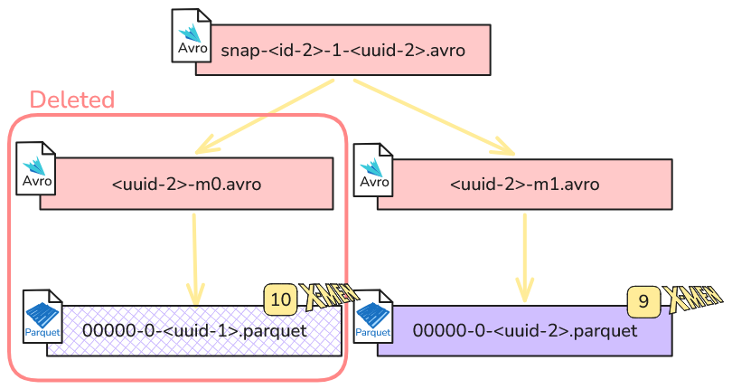
We got this result, because per default the write.delete.mode of our Iceberg table is set to copy-on-write. In this mode the writer has to do the heavy lifting and whole data files are copied and rewritten. But Iceberg allows to change this behavior.

Merge-on-read

Let's rewind time, and delete Cyclops again, but this time with the merge-on-read mode. For this we first have to alter our table properties, using

spark.sql("ALTER TABLE marvel.xmen.characters SET TBLPROPERTIES ('write.delete.mode' = 'merge-on-read')")

and then delete Cyclops again

spark.sql("DELETE FROM marvel.xmen.characters WHERE id = 1")

As always, we check the filesystem structure to see what happened:

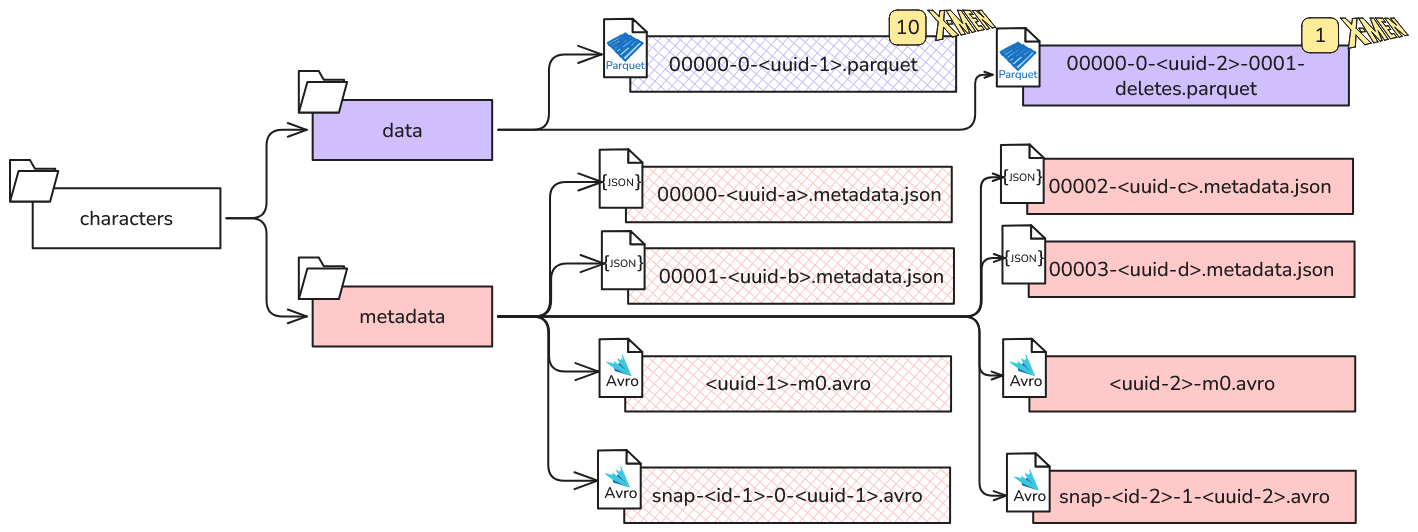
We now have a delete file! Also, we have an additional metadata file, which captures the change of the write.delete.mode. Inspecting the latest snapshot we see the following hierarchy:

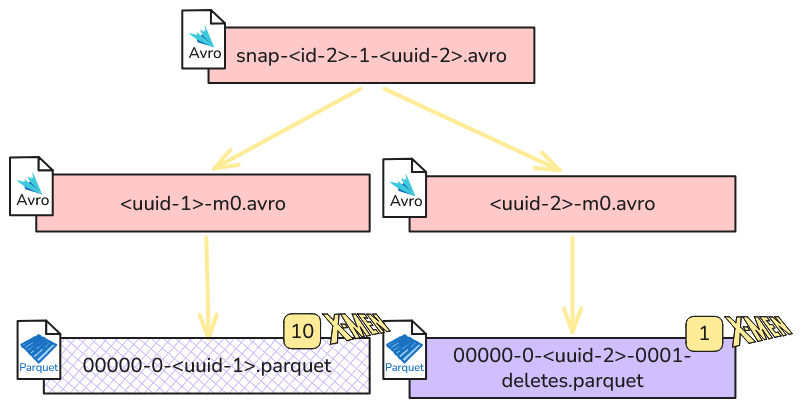
Now when the table is accessed the reader has to do the heavy lifting. It must first load the data file and then the delete file, which in our case looks like this:

+------------------------------------------------------------------+-------+
| file_path                                                        |   pos |
|------------------------------------------------------------------+-------|
| file:/tmp/warehouse/xmen/characters/data/00000-0-<uuid-1>.parquet|     0 |
+------------------------------------------------------------------+-------+

It just states what position, 0, in what file, 00000-0-<uuid-1>.parquet, should be deleted, which is why this kind of delete files are called a position delete files. The actual data is then "merged" with the delete file to remove Cyclops, and yield the final table with nine X-Men. In practice the process is a bit more complicated, but in its gist this is how it works.

Deletion vectors

At this point it is a good time to talk about the different versions of the Apache Iceberg specification, because position delete files have been deprecated in v3 and been replaced by deletion vectors. A new version of the specification is introduced when features are added that would break forward compatibility, i.e. old readers can no longer correctly read tables using new features. When writing this blog post v1, v2 and v3 have been released, while v4 is in active development. The most confusing part for versions is that there is a heavy discrepancy on feature implementation status between the different implementations. The status can be compared here, where the Java implementation is always the most complete one and leads direction. But others like PyIceberg are trying to keep up, see for example their progress on implementing all features for v3.

To showcase this let's do another example for deletion vectors and rewind time again! When we started out creating our xmen table the version defaulted to v2, because we used PyIceberg for it. The available features are bound to the version of the table, and therefore even if we use PySpark to delete Cyclops, which uses the v3 compatible Java implementation, we will not produce a deletion vector. But we can upgrade the version of a table by changing its properties, which can be done using:

spark.sql("""
    ALTER TABLE marvel.xmen.characters
    SET TBLPROPERTIES ('format-version' = '3',
                       'write.delete.mode' = 'merge-on-read'
    )
""")

To ensure that this worked we can inspect the table properties:

df = spark.sql("SHOW TBLPROPERTIES marvel.xmen.characters")
df.show()

to see

+-------------------+-------------------+
|                key|              value|
+-------------------+-------------------+
|current-snapshot-id|             <id-2>|
|             format|    iceberg/parquet|
|     format-version|                  3|
|  write.delete.mode|      merge-on-read|
+-------------------+-------------------+

Then we delete Cyclops again

spark.sql("DELETE FROM marvel.xmen.characters WHERE id = 1")

The file setup is now identical to the previous v2 delete, but we get a puffin delete file 00000-0-<uuid-2>-0001-deletes.puffin instead of a parquet one. The big difference here is that a position delete file stores one line per deleted row and that there can be many delete files associated with a single data file. For example if we would delete more and more X-Men one by one, we would create a new delete file for each deletion. This accumulates work for a reader, having to scan many delete files, leading to a bad performance. In contrary a deletion vector is a bitmap that encodes what rows are deleted, i.e. an array of bits, one for each row of the associated data file, where a 1 indicates that this record is deleted. Additionally the v3 specification states that writes have to make sure that only one deletion vector exists for any data file. Hence, a delete is now no longer a file creation operation, but a bitmap modification operation. For more infos on this see here.

Let's have a look at the puffin file, which is in its gist just storing an array of blobs and a JSON, that describes how to interpret these blobs. In our case the JSON looks like this:

{
  "blobs": [
    {
      "type": "deletion-vector-v1",
      "fields": [
        2147483645
      ],
      "snapshot-id": -1,
      "sequence-number": -1,
      "offset": 4,
      "length": 42,
      "properties": {
        "referenced-data-file": "file:///tmp/warehouse/xmen/characters/data/00000-0-<uuid-1>.parquet",
        "cardinality": "1"
      }
    }
  ],
  "properties": {
    "created-by": "Apache Iceberg 1.10.0 (commit 2114bf631e49af532d66e2ce148ee49dd1dd1f1f)"
  }
}

This tell us that the blob at offset 4 is a deletion-vector-v1 type, which references the data file 00000-0-<uuid-1>.parquet and deletes a single row (cardinality: 1). To actually know which row was deleted, i.e. checking which bit is 1 in the bitmap, a reader would now need to decode the blob.

Equality delete files

As probably already suspected, position delete files are not the only kind of delete files, there are also equality delete files. In contrast, they do not delete rows by indiviually referencing them, but state a specific column-value combination, and all rows that match it should be deleted. The reader is then responsible to select these rows and discard them from the table.

I was unable to "force" PySpark to do a equality delete, it seems to prefer deleting by position. Therefore I opted for iceberg-rust to manually create a equality delete file, which you can find here. To spare you the details, I deleted all inactive x-men, i.e. deleting all rows where the field active=false. This simply yielded the file delete-00000.parquet, which looks as follows:

+----------+
|   active |
|----------|
|        0 |
+----------+

Example: Update an X-Man

Similar to a delete, we can use Apache Icebergs merge-on-read mode to update a single X-Man. Starting from our base line table we again need to change the write.update.mode:

spark.sql("""
    ALTER TABLE marvel.xmen.characters
    SET TBLPROPERTIES (
        'write.update.mode' = 'merge-on-read',
        'format-version' = '2'
    )
""")

and then due to some beef with Wolverine, Cyclops decides to stop being an X-Man and we update him:

spark.sql("""
    UPDATE marvel.xmen.characters
    SET active = false
    WHERE id = 1
""")

This yields the following filesystem structure:

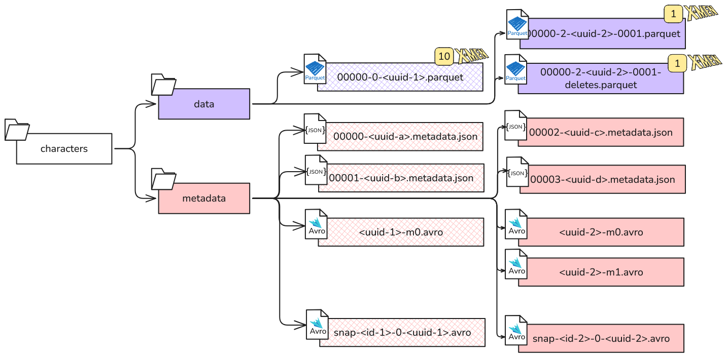
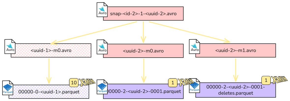
We created a delete file that deletes the initial row for Cyclops and a data file that holds his new active status. In addition a manifest file was created for each of the new data/delete files. The latest snapshot now points to all existing manifest files, which in combination show the desired state of the table.

Example: Schema evolution

When we initially looked at one of the metadata JSON files of our Iceberg table, you may have noticed the fields called schemas with list type and current-schema-id with an int type. These are reminiscent of the snapshots and current-snapshot-id fields, but instead of allowing our table to change over time, allow the schema of the table to change. This change is called schema evolution, and this example shows how it works.

We start of with our base table with the known schema:

table = catalog.load_table("xmen.characters")
print(table.schema())

table {
  1: id: optional long
  2: name: optional string
  3: alias: optional string
  4: powers: optional string
  5: birth_year: optional long
  6: active: optional boolean
}

Now PyIceberg allows us to alter the schema via methods, for example re-naming, adding or changing the order of columns:

with table.update_schema() as update:
    update.rename_column("alias", "codename")
    update.add_column("first_appearance", StringType())
    update.move_after("active", "first_appearance")

Now we can add new X-Men that follow this new schema of the table:

df = read_csv("./x-men3.csv")
table.append(df)

and if we take a look at it

print(table.scan().to_pandas())

we see the following:

id              name      codename                                      powers  birth_year         first_appearance  active
11  Illyana Rasputin         Magik  Teleportation through Limbo and dark magic        1982      Giant-Size X-Men #1    True
12  Roberto da Costa       Sunspot  Solar energy absorption and super strength        1984  Marvel Graphic Novel #4    True
 1     Scott Summers       Cyclops               Optic blasts, team leadership        1970                      NaN    True
 2         Jean Grey       Phoenix       Telepathy, telekinesis, Phoenix Force        1972                      NaN    True

Notice, that the schema has changed and that for the new column first_appearance, that was none existing for the old data we wrote, we simply get a NaN value.

How does this work? Under the hood the first parquet file that we wrote has not changed. It still has the original schema, with the alias column.

+------+-----------------+--------------+-----------+--------------+----------+
|   id | name            | alias        | powers    |   birth_year | active   |
|------+-----------------+--------------+-----------+--------------+----------|
|    1 | Scott Summers   | Cyclops      | [...]     |         1970 | True     |
|    2 | Jean Grey       | Phoenix      | [...]     |         1972 | True     |
[...]

In contrast the new parquet file has the re-named column codename instead and the new column first_appearance right before the active column:

+------+------------------+------------+--------+--------------+-------------------------+----------+
|   id | name             | codename   | powers |   birth_year | first_appearance        | active   |
|------+------------------+------------+--------+--------------+-------------------------+----------|
|   11 | Illyana Rasputin | Magik      | [...]  |         1982 | Giant-Size X-Men #1     | True     |
|   12 | Roberto da Costa | Sunspot    | [...]  |         1984 | Marvel Graphic Novel #4 | True     |
+------+------------------+------------+--------+--------------+-------------------------+----------+

Without Apache Iceberg these parquet files would be incompatible. If the reader you choose to view them is positioned based the columns no longer line up and the data types are even different. For a name based reader one could match the existing values for the active column and just show NaN for the new first_appearance column. But because of the re-name alias -> codename the reader could not make sense of the change.

Apache Iceberg fixes this by not being based on position or name, but instead referencing fields by id. If we take a look at the new metadata file that has been produced, we will see that schemas now has two entries:

"schemas": [
  {
    "type": "struct",
    "fields": [
      {
        "id": 1,
        "name": "id",
        "type": "long",
        "required": false
      },
      {
        "id": 2,
        "name": "name",
        "type": "string",
        "required": false
      },
      {
        "id": 3,
        "name": "alias",
        "type": "string",
        "required": false
      },
      {
        "id": 4,
        "name": "powers",
        "type": "string",
        "required": false
      },
      {
        "id": 5,
        "name": "birth_year",
        "type": "long",
        "required": false
      },
      {
        "id": 6,
        "name": "active",
        "type": "boolean",
        "required": false
      }
    ],
    "schema-id": 0,
    "identifier-field-ids": []
  },
  {
    "type": "struct",
    "fields": [
      {
        "id": 1,
        "name": "id",
        "type": "long",
        "required": false
      },
      {
        "id": 2,
        "name": "name",
        "type": "string",
        "required": false
      },
      {
        "id": 3,
        "name": "codename",
        "type": "string",
        "required": false
      },
      {
        "id": 4,
        "name": "powers",
        "type": "string",
        "required": false
      },
      {
        "id": 5,
        "name": "birth_year",
        "type": "long",
        "required": false
      },
      {
        "id": 7,
        "name": "first_appearance",
        "type": "string",
        "required": false
      },
      {
        "id": 6,
        "name": "active",
        "type": "boolean",
        "required": false
      }
    ],
    "schema-id": 1,
    "identifier-field-ids": []
  }
]

Here every field has an id, and we can see that the field with id 3 had the name alias in the first version and in the latest it is called codename. Now if we inspect the file metadata of our parquet files using

parquet-tools meta ./data/00000-0-<uuid-2>.parquet | jq

we find inside each SchemaElement a FieldID. For example for the codename column we get the following for the new parquet file:

{
  "PathInSchema": [
    "codename"
  ],
  [...]
  "FieldID": 3,
  [...]
},

When appending the data, the PyIceberg writer took care of embedding these file ids into the data file. This way when a reader now scans the table it can project the data of the underlying data files onto the most recent schema, even through they may have been written with an older one.

Example: Partitioning

In the old Hive way partitions were solely encoded in the directory path, e.g. /year=2026/month=08/day=13. This goes by the name of hive style partitioning. While it is straight forward, there are two downsides to it: First, the data values are directly used in the path, which can lead to errors depending on the storage for special characters like spaces or slashes. Second, the partitioning scheme is directly encoded in the path structure, with no intermediate layer. This way for every change in the partitioning of the data, the path structure needs to change.

The first downsides is nicley handled in Apache Iceberg by URL encoding special characters. Let's look at this for some X-Men with special characters in their aliases:

id	name	alias	powers	birth_year	active
1	Warren Kenneth Worthington III	Angel/Archangel	Flight with feathered wings, aerial combat	1963	TRUE
2	Kevin Sydney	Changeling=Morph	Shapeshifting, Psionic powers, Skilled actor	1968	FALSE

Here we will just partition on the value of the alias field, without changing it, i.e. we use an identity transformation:

from pyiceberg.partitioning import PartitionField, PartitionSpec
from pyiceberg.transforms import IdentityTransform

partition_spec = PartitionSpec(
    PartitionField(
        source_id=3, field_id=1000, transform=IdentityTransform(), name="alias"
    )
)
table = catalog.create_table(
    identifier="xmen.characters",
    schema=schema,
    partition_spec=partition_spec,
)
table.append(df)

This yields the following filesystem structure:

$ tree
.
├── pyiceberg_catalog.db
└── xmen
    └── characters
        ├── data
        │   ├── alias=Angel%2FArchangel
        │   │   └── 00000-0-<uuid-1>.parquet
        │   └── alias=Changeling%3DMorph
        │       └── 00000-1-<uuid-1>.parquet
        └── metadata
            ├── 00000-<uuid-a>.metadata.json
            ├── 00001-<uuid-b>.metadata.json
            ├── <uuid-1>-m0.avro
            └── snap-<id-1>-0-<uuid-1>.avro

The special characters are safely encoded: / -> %2F and = -> %3D.

This is nice, but the far bigger feature is that Iceberg actually decouples the partitioning of a table from its physical layout, which solves the second downside. When we created the table the information of the partition spec is stored in the metadata file:

"partition-specs": [
    {
      "spec-id": 0,
      "fields": [
        {
          "source-id": 3,
          "field-id": 1000,
          "transform": "identity",
          "name": "alias"
        }
      ]
    }
  ]

If we now come to the conclusion that using the full alias for partitioning our X-Men table may not be that smart, we can just change it. For example we could delete our identity transformation and partition by the first letter of the alias by using the TruncateTransform:

from pyiceberg.transforms import TruncateTransform

with table.update_spec() as update:
    update.remove_field("alias")
    update.add_field("alias", TruncateTransform(1), "alias_truncated")

For other transformations see the spec here.

If we now append more X-Men using

df = read_csv("./x-men.csv")
table.append(df)

the filesystem structure changes to

$ tree
.
├── pyiceberg_catalog.db
└── xmen
    └── characters
        ├── data
        │   ├── alias=Angel%2FArchangel
        │   │   └── 00000-0-<uuid-1>.parquet
        │   ├── alias=Changeling%3DMorph
        │   │   └── 00000-1-<uuid-1>.parquet
        │   ├── alias_truncated=B
        │   │   └── 00000-4-<uuid-2>.parquet
        │   ├── alias_truncated=C
        │   │   └── 00000-0-<uuid-2>.parquet
        │   ├── alias_truncated=N
        │   │   └── 00000-5-<uuid-2>.parquet
        │   ├── alias_truncated=P
        │   │   └── 00000-1-<uuid-2>.parquet
        │   ├── alias_truncated=Q
        │   │   └── 00000-6-<uuid-2>.parquet
        │   ├── alias_truncated=R
        │   │   └── 00000-7-<uuid-2>.parquet
        │   ├── alias_truncated=S
        │   │   └── 00000-3-<uuid-2>.parquet
        │   └── alias_truncated=W
        │       └── 00000-2-<uuid-2>.parquet
        └── metadata
            ├── 00000-<uuid-a>.metadata.json
            ├── 00001-<uuid-b>.metadata.json
            ├── 00002-<uuid-c>.metadata.json
            ├── 00003-<uuid-d>.metadata.json
            ├── <uuid-1>-m0.avro
            ├── <uuid-2>-m0.avro
            ├── snap-<id-2>-0-<uuid-2>.avro
            └── snap-<id-1>-0-<uuid-1>.avro

We see that the old partitions are still there, but for the new records the new partition spec was used. The most recent metadata file now contains a new partition spec

"partition-specs": [
    {
      "spec-id": 0,
      "fields": [
        {
          "source-id": 3,
          "field-id": 1000,
          "transform": "identity",
          "name": "alias"
        }
      ]
    },
    {
      "spec-id": 1,
      "fields": [
        {
          "source-id": 3,
          "field-id": 1001,
          "transform": "truncate[1]",
          "name": "alias_truncated"
        }
      ]
    }
  ]

and the latest manifest list file states what partition spec was used to create which manifest file:

{
  "manifest_path": "file:///tmp/warehouse/xmen/characters/metadata/<uuid-2>-m0.avro",
  "manifest_length": 7325,
  "partition_spec_id": 1,
    [...]
}
{
  "manifest_path": "file:///tmp/warehouse/xmen/characters/metadata/<uuid-1>-m0.avro",
  "manifest_length": 5268,
  "partition_spec_id": 0,
    [...]
}

The concept of decoupling logical from physical layout is similar to the previous schema evolution section. In short it allows a reader to still understand the "old way" of partitioning our data, while a writer can write new data with the new spec. To show this we can look at what happens if we want to filter for X-men, who's alias starts with a "C":

scan = table.scan(row_filter="alias like 'C%'")

Then we can look at the files that reader identified:

tasks = scan.plan_files()

and printing them yields:

================================================================================
Files to read:
================================================================================

File: file:///tmp/warehouse/xmen/characters/data/alias_truncated=C/00000-0-<uuid-2>.parquet
  Partition: Record[C]
  Record count: 1
  File size: 2416 bytes
  Spec ID: 1

File: file:///tmp/warehouse/xmen/characters/data/alias=Changeling%3DMorph/00000-1-<uuid-1>.parquet
  Partition: Record[Changeling=Morph]
  Record count: 1
  File size: 2531 bytes
  Spec ID: 0

================================================================================
Query Results:
================================================================================
   id           name             alias                                        powers  birth_year  active
0   1  Scott Summers           Cyclops                 Optic blasts, team leadership        1970    True
1   2   Kevin Sydney  Changeling=Morph  Shapeshifting, Psionic powers, Skilled actor        1968   False

Hence the reader understood both partitioning spec and found the correct files to read.

Example: Tags, branches and time travel

During the last examples we have seen how Apache Icebergs metadata layer enables multiple features. One key insight was, that an Iceberg table not only stores what data currently makes up a table, but what operations lead to this state, and how previous states looked in the form of snapshots. To capitalize on all of this Apache Icebergs give the tools to navigate snapshots in the form of tags, branches and time travel.

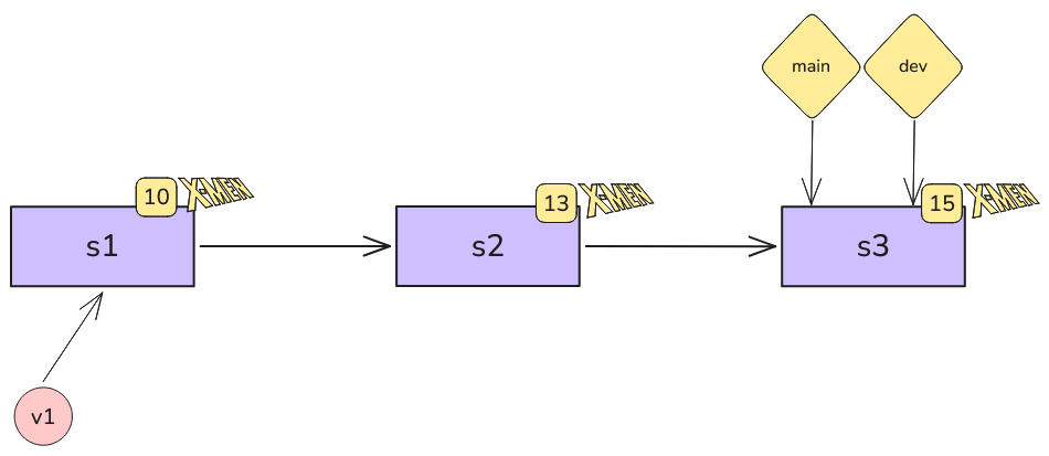
As always we start with our base table with ten X-Men, which is our snapshot s1. We can now create a tag for this snapshot, where a tag is just a name, to reference a snapshot instead of using it's id:

table.manage_snapshots().create_tag(
    snapshot_id=table.current_snapshot().snapshot_id, tag_name="v1"
).commit()

In the metadata file this shows up like this:

"refs": {
    "main": {
      "snapshot-id": s1,
      "type": "branch"
    },
    "v1": {
      "snapshot-id": s1,
      "type": "tag"
    }
}

Now we can add three more X-Men to create a another snapshot:

df = read_csv("./x-men2.csv")
table.append(df)
print(len(table.scan().to_arrow()))
# > 13

Notice now, that in the metadata file there is always a thing called main branch. This is the current state of the table and we can see that it now points to the latest snapshot, while the tag v1 still points to the old one:

"refs": {
    "main": {
      "snapshot-id": s2,
      "type": "branch"
    },
    "v1": {
      "snapshot-id": s1,
      "type": "tag"
    },
}

Visually we can represent this as

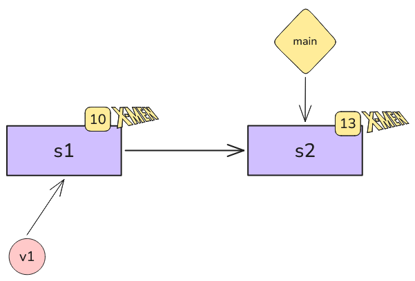
The key idea is, that the old snapshot s1 still exists. By adding new data nothing was overwritten, no information of how we ended up in this state was lost. Everything is still there, captured in the hierarchy of metadata files. Therefore we can just query an older state of the table if we want to:

v1_snapshot_id = table.refs()["v1"].snapshot_id
print(len(table.scan(snapshot_id=v1_snapshot_id).to_arrow()))
# > 10

This feature of looking at a previous state of a table goes by the name of time travel. Typically this feature is showcased by running a query for a table as it looked like at a specific point in time, e.g.

SELECT count(*) FROM xmen.characters TIMESTAMP AS OF '2026-08-16 22:45:00'

But note, that this does not magically offer to travel time freely. Behind the scenes just the snapshot with a timestamp closest before the given timestamp is selected, see the offical PyIceberg docs:

def snapshot_as_of_timestamp(self, timestamp_ms: int, inclusive: bool = True) -> Snapshot | None:
    """Get the snapshot that was current as of or right before the given timestamp, or None if there is no matching snapshot.

Hence, if your data has some kind of creation time semantics that differ from how you commit new data to the Iceberg table, you may get suprising results.

Anyways, let's now create a new branch. In contrast to tags, branches are not bound to a single snapshot, but move. When new data is committed to them, and with it a new snapshot created, they automatically update to point to this new snapshot. In the end this is just like git branches behaves. (And thinking about it, Apache Iceberg in general shares a lot of similarities with git. See here for a nice git deep dive.)

We can create a new branch via:

table.manage_snapshots().create_branch(
    snapshot_id=table.current_snapshot().snapshot_id, branch_name="dev"
).commit()

And then only append two more X-Men to this branch

df = read_csv("./x-men4.csv")
table.append(df, branch="dev")
print(len(table.scan().to_arrow()))
# > 13

What happened now is that a new snapshot was created but only the dev branch references it:

"refs": {
  "main": {
    "snapshot-id": s2,
    "type": "branch"
  },
  "v1": {
    "snapshot-id": s1,
    "type": "tag"
  },
  "dev": {
    "snapshot-id": s3,
    "type": "branch"
  }
},

Visually we can represent this as

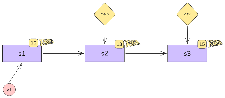
This branch feature is perfect for patterns like the write-audit-publish pattern. In this pattern new data is first written, then it is checked if it matches the data quality requirements (audit), and the depending on the output of the audit it is either published, i.e. declared the new state of the table or dismissed. In this spirit, Iceberg allows us to query the latest newly written, but yet unpublished data, via

dev_snapshot_id = table.refs()["dev"].snapshot_id
audit_scan = table.scan(snapshot_id=dev_snapshot_id).to_arrow()

on which we could run some data quality checks. And if they all passed we could publish them, i.e. set the current snapshot of the table to it, using.

table.manage_snapshots().set_current_snapshot(ref_name="dev").commit()

Then when querying the default state of the table, we now see the full 15 X-Men:

print(len(table.scan().to_arrow()))
# > 15

Visually we can represent this as

Example: Maintenance

We have now seen that Apache Iceberg brings many features that systematically improve on weaknesses of Hive tables. But, as always, there is no free lunch. To make all these features possible, Iceberg tables must do a lot of heavy lifting. Every change of data, be it an append, delete or update, requires multiple metadata files to be written in addition to the actual data files. Also, depending on what write mode is used, much redundant data may be written and stored indefinitely. Down the line, just normally using Iceberg tables can lead to shortcomings like wasted storage, reading many small data files or cumbersome scanning through many metadata files. To combat this PySpark supplies a set of maintenance operations.

For this section we will start with the previous example as our baseline, i.e. three snapshots for which we append first ten, then three and then two X-Men.

The first thing we can do is reduce the number of metadata files. As stated before, one of the big advantage of Iceberg is that it reduces the number of API calls needed for planning a scan by containing multiple file paths in a single manifest file. But if we store a single manifest file for each data file this advantage is lost. To avoid this we can rewrite manifest files using:

spark.sql(""" CALL marvel.system.rewrite_manifests('xmen.characters') """).show()

+-------------------------+---------------------+
|rewritten_manifests_count|added_manifests_count|
+-------------------------+---------------------+
|                        3|                    1|
+-------------------------+---------------------+

Which leaves us with a single manifest file that references all data files.

The second thing we can do is to combine multiple small data files into bigger ones, a technique called compaction. While this does not matter for our toy data set example, for production environments one usually aims for data files of around 512 MB (the default target data file size when compacting). This number is not chosen arbitrarily, but is a sweet spot when balancing multiple opposing incentives. On one side large files are favored, because:

Each data size contains necessary metadata information, i.e. headers and footers. The larger the data file the lower (better) the storage amplification. Storage amplification means here, that one needs to write things like headers/footers in addition to the data one actually wants to write, i.e. row groups.
As the data files are usually accessed via a network the API call overhead per file can add up. (Same issue as with scan planning). Having bigger and therefore less files reduces this overhead.

On the other side small files are favored, because:

Each file can be worked on in parallel by a worker of the query engine used. With more smaller files the workload can be better parallelized.
As files are typically processed by workers in memory the content of a file should fit inside the memory of a worker. Due to typical resource allocation in a query engine cluster this poses a limit on how big a file should get.

Considering these factors, data files around 512 MB have just proven themselves to be efficient in practice for common applications.

To actually compact our data files we can call the following:

spark.sql(
    """ CALL marvel.system.rewrite_data_files(table => 'xmen.characters', options => map('rewrite-all', 'true')) """
).show()

# +--------------------------+----------------------+---------------------+-----------------------+--------------------------+
# |rewritten_data_files_count|added_data_files_count|rewritten_bytes_count|failed_data_files_count|removed_delete_files_count|
# +--------------------------+----------------------+---------------------+-----------------------+--------------------------+
# |                         3|                     1|                 8131|                      0|                         0|
# +--------------------------+----------------------+---------------------+-----------------------+--------------------------+

Which leaves us with a single data file, which also simplifies the latest manifest file.

The last maintenance step I want to show is the expiration of snapshots. As almost every operation on an iceberg table creates a new snapshots many manifest list files accumulate over time. Depending on the frequency and granularity with which one appends or deletes data from an Iceberg table, keeping all these snapshots may not be needed and just waste storage. Therefore one can simply expire old snapshots and automatically get rid of data and manifest files that are only references in the expired snapshots.

Due to our two previous maintenance operation the current filesystem structure looks as follows:

/tmp/warehouse
$ tree
.
├── pyiceberg_catalog.db
└── xmen
    └── characters
        ├── data
        │   ├── 00000-0-<uuid-1>.parquet
        │   ├── 00000-0-<uuid-2>.parquet
        │   ├── 00000-0-<uuid-3>.parquet
        │   └── 00000-5-eb8d5a9d-a6d6-48df-ab22-3387a3426791-0-00001.parquet
        └── metadata
            ├── 00000-<uuid-a>.metadata.json
            ├── 00001-<uuid-b>.metadata.json
            ├── 00002-<uuid-c>.metadata.json
            ├── 00003-<uuid-d>.metadata.json
            ├── 00004-<uuid-e>.metadata.json
            ├── 00005-<uuid-f>.metadata.json
            ├── 00006-<uuid-g>.metadata.json
            ├── 00007-<uuid-h>.metadata.json
            ├── 00008-<uuid-i>.metadata.json
            ├── <uuid-1>-m0.avro
            ├── <uuid-2>-m0.avro
            ├── <uuid-5>-m0.avro
            ├── <uuid-5>-m1.avro
            ├── <uuid-3>-m0.avro
            ├── optimized-m-463ec091-f9ac-4a0f-8a3a-e65617563e55.avro
            ├── snap-3014518774835702005-1-<uuid-4>.avro
            ├── snap-4956052972558252728-0-<uuid-3>.avro
            ├── snap-768964918616401465-1-<uuid-5>.avro
            ├── snap-8380523983098070968-0-<uuid-2>.avro
            └── snap-9164814029224031324-0-<uuid-1>.avro

We now expire all snapshots older than a future date (so all), but want retain at least one using

spark.sql(
    """ CALL marvel.system.expire_snapshots('xmen.characters', TIMESTAMP '2044-08-18 00:00:00.000', 1); """
).show()

The summary gives us information on what data and metadata files could be deleted by expiring snapshots:

+------------------------+-----------------------------------+-----------------------------------+----------------------------+----------------------------+------------------------------+
|deleted_data_files_count|deleted_position_delete_files_count|deleted_equality_delete_files_count|deleted_manifest_files_count|deleted_manifest_lists_count|deleted_statistics_files_count|
+------------------------+-----------------------------------+-----------------------------------+----------------------------+----------------------------+------------------------------+
|                       0|                                  0|                                  0|                           1|                           2|                             0|
+------------------------+-----------------------------------+-----------------------------------+----------------------------+----------------------------+------------------------------+

Finally we have the following filesystem structure:

$ tree
.
├── pyiceberg_catalog.db
└── xmen
    └── characters
        ├── data
        │   ├── 00000-0-<uuid-1>.parquet
        │   ├── 00000-0-<uuid-2>.parquet
        │   ├── 00000-0-<uuid-3>.parquet
        │   └── 00000-5-eb8d5a9d-a6d6-48df-ab22-3387a3426791-0-00001.parquet
        └── metadata
            ├── 00000-<uuid-a>.metadata.json
            ├── 00001-<uuid-b>.metadata.json
            ├── 00002-<uuid-c>.metadata.json
            ├── 00003-<uuid-d>.metadata.json
            ├── 00004-<uuid-e>.metadata.json
            ├── 00005-<uuid-f>.metadata.json
            ├── 00006-<uuid-g>.metadata.json
            ├── 00007-<uuid-h>.metadata.json
            ├── 00008-<uuid-i>.metadata.json
            ├── 00009-<uuid-j>.metadata.json
            ├── <uuid-1>-m0.avro
            ├── <uuid-2>-m0.avro
            ├── <uuid-5>-m0.avro
            ├── <uuid-5>-m1.avro
            ├── <uuid-3>-m0.avro
            ├── snap-4956052972558252728-0-<uuid-3>.avro
            ├── snap-768964918616401465-1-<uuid-5>.avro
            └── snap-9164814029224031324-0-<uuid-1>.avro

Here we see that actually three snapshots still remain in our iceberg table. This is because snapshots, which are referenced by tag or branch, in our case the tag v1 and the branch dev, are protected from expiration.

Closing

We covered a lot of ground and covered the most important features of Apache Iceberg from the ground up. I hope reading this post lifted some mysteries of Apache Iceberg for you. In writing this I sure learned a lot! If you want to dig deeper and see everything Apache Iceberg has to offer, there is not better place than the official specification.

Grokking Apache Iceberg

Table of Contents

Apache Iceberg in a nutshell

The old Hive way

Hive demonstration

Other shortcomings

Core ideas

The data layer

The metadata layer

The data catalog layer

Examples

Example: Create an Iceberg table and show file structure

Example: Append more X-Men

Example: Delete an X-Man

Copy-on-write

Merge-on-read

Deletion vectors

Equality delete files

Example: Update an X-Man

Example: Schema evolution

Example: Partitioning

Example: Tags, branches and time travel

Example: Maintenance

Closing